

Decoupled Single-Mask Annotation Noise Detection via Cross-Sectional Patch Self-Consistency
Yinheng Zhu1 and Xiaowei Xu2,✉
1 Tsinghua University, Beijing, China
2 Guangdong Provincial People's Hospital, Guangzhou, China
✉ corresponding author
Medical Image Computing and Computer Assisted Intervention
(MICCAI) 2026
Oral Poster
Annotation noise is not random
Vascular CT is usually annotated once per scan, because repeated expert labelling is
costly. A single mask leaves nothing to compare it against, so it is hard to say which
parts of it are wrong. We proposed a way
We found that annotation noise correlates strongly with the direction a vessel runs. Below is the noise rate over vessel direction: how often a cross-section is flagged, as a function of which way it points. The six poles are the imaging axes. The rate dips there, and those are the cleanest annotations. The bulges between them are vessels running diagonally through the scanner.
Loading direction data…
Measured as the angular distance θ to the nearest imaging axis, the rate rises close
to monotonically across the range, from 0.44% at θ ≈ 0° to 2.24%
at θ ≈ 55°. Spearman ρ = −0.20;
Cochran–Armitage trend test
And not only orientation
Annotation noise also correlates with cross-sectional area and with intensity, and these two share one cause. Cross-sections under 2 mm² show markedly elevated noise rates, declining rapidly beyond 5 mm². The rate also peaks below 0 HU, at approximately 5–6%, and drops through the typical lumen range of 50–200 HU. Thin vessels occupy only a few pixels in axial slices, and low contrast leaves less separation between vessel wall and background. Both trends reflect the same condition: reduced boundary discriminability at annotation time.
Our explanation for these findings is that it may correlate with the annotation tools.
Annotation is done slice by slice, in tools such as
ITK-SNAP
The principle and auditable evidence
A single pair of cross-sections, drawn from two different scans, states the problem the method addresses.
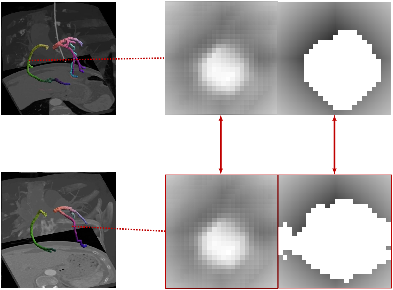 Same image.
Different mask.
Same image.
Different mask.
Existing approaches fall into two families. Multi-rater
fusion
Tubular anatomy provides option (b). Sampled perpendicular to the centreline, cross-sections recur along the same vessel and across different subjects, so the dataset already contains its own near-repeats without any additional annotation. The principle then needs one word relaxed, from the same image to a near-identical one:
dI(Ii, Ij) ≤ εI ⇒ dM(Mi, Mj) ≤ εM
Image distance dI is mean squared error; mask distance dM is one minus intersection over union. Each patch is compared with every neighbour retrieved within εI, and the median of those pair scores gives its patch-level score Ri: a signed z-score of mask disagreement, calibrated against how much disagreement is normal for pairs of that similarity. A patch whose mask disagrees with most of its retrieved neighbours is driven to Ri << 0.
The criterion is computed directly from the image–mask pair rather than from network behaviour, so each flagged region is surfaced together with the retrieved neighbours that produced its score. This is what the work set out to provide: in a single-rater dataset, annotation noise identified decoupled from training, on auditable evidence. The demo below steps along one centreline and shows the retrieved neighbours at each cross-section.
Loading scan…
Retrieved neighbours that set this score, ordered by mask disagreement. A trailing * marks one from a different scan.
← mask agreesmask disagrees →
The score is graded rather than binary: it separates severe disagreement from mild boundary shifts, and it also identifies clean annotation as clean.
Loading spectrum…
How it works
The pipeline has three stages, none of which involves training a network.
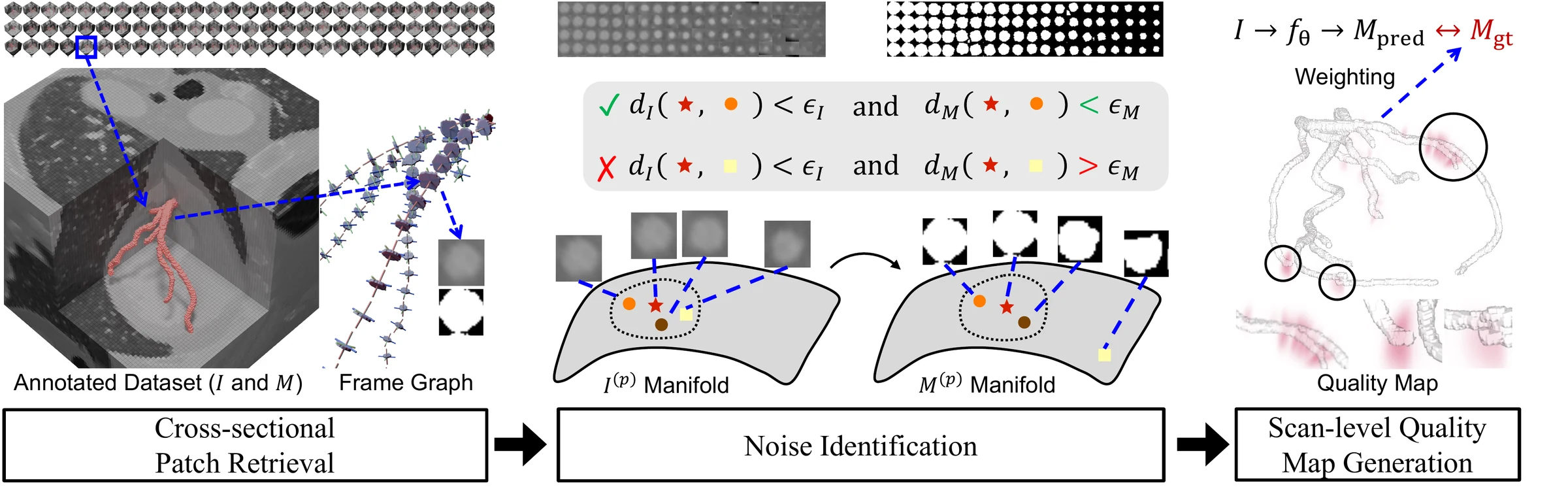
- Sample patches along the centreline.
- 103 volumes produce ∼3×10⁶ patches.
- Bishop frames
keep them stable.
- Operationalise the principle as a statistical test.
-
Implemented with a vector search engine
to accommodate 106+6 patch pairs.
- Spread patch residuals onto voxels to obtain a quality map for loss weighting.
Three choices deserve comment. The frames are torsion-free: a frame that twists as it travels would rotate the patch with it, and a rotated cross-section is no longer retrievable as near-identical, which would cost the method the pairs it depends on. The retrieval tolerance εI = 10−3 MSE corresponds to about 30 dB PSNR, the level at which two patches stop being distinguishable by eye, which is what licenses treating a retrieved neighbour as the same image. And mask disagreement is not compared against a fixed threshold: pairs are binned by image distance and calibrated within each bin, so a pair is judged against the disagreement that is normal at its own level of similarity.
Failure cases and limitations
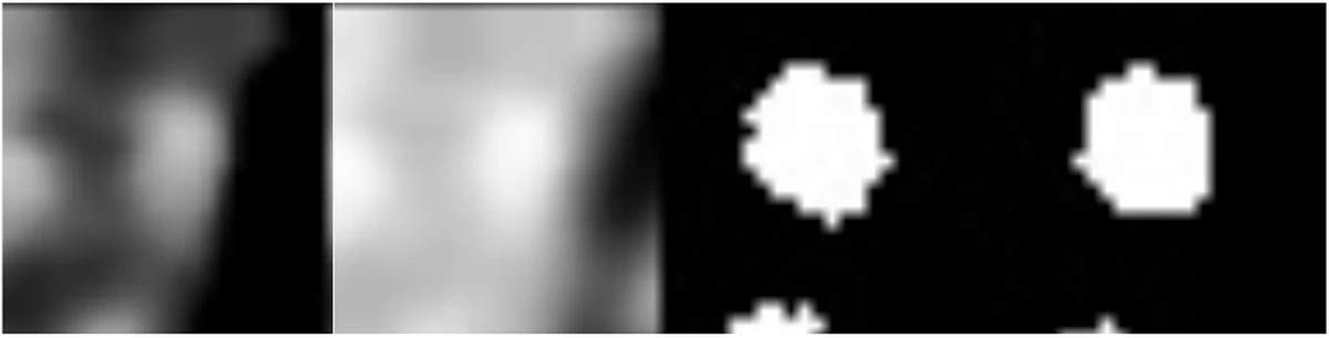
The dominant failure pattern is false negatives. Noise goes undetected when no sufficiently similar counterpart is retrieved: patches that are near-identical only up to a rotation, or up to a window-level shift, are missed by raw-MSE retrieval. Centreline and frame errors have the same effect. All of these reduce recall rather than precision, which is the trade the design prioritises. Recall is recoverable by denser sampling of rotations and shifts, at higher computational cost.
The method detects rather than corrects noise, assumes tubular anatomy, and has been
evaluated on ImageCAS

References
How to cite
@inproceedings{zhu2026hiddennoise,
  title     = {Decoupled Single-Mask Annotation Noise Detection via
               Cross-Sectional Patch Self-Consistency},
  author    = {Zhu, Yinheng and Xu, Xiaowei},
  booktitle = {Medical Image Computing and Computer Assisted Intervention
               (MICCAI)},
  year      = {2026},
  eprint    = {2607.05965},
  archivePrefix = {arXiv},
}
Acknowledgements
Experiments use the ImageCAS coronary CT angiography dataset.